1
2
3
4
5
6
7
8
9
10
11
12
13
14
15
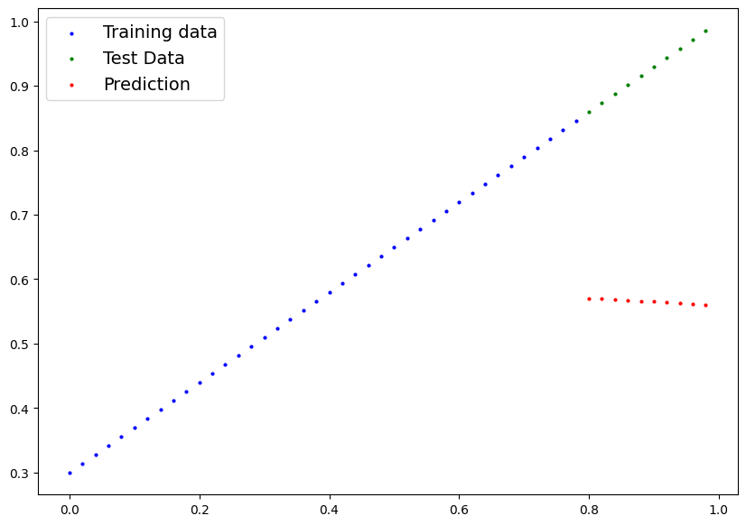
| X
-->tensor([0.0000, 0.0200, 0.0400, 0.0600, 0.0800, 0.1000, 0.1200, 0.1400, 0.1600,
0.1800, 0.2000, 0.2200, 0.2400, 0.2600, 0.2800, 0.3000, 0.3200, 0.3400,
0.3600, 0.3800, 0.4000, 0.4200, 0.4400, 0.4600, 0.4800, 0.5000, 0.5200,
0.5400, 0.5600, 0.5800, 0.6000, 0.6200, 0.6400, 0.6600, 0.6800, 0.7000,
0.7200, 0.7400, 0.7600, 0.7800, 0.8000, 0.8200, 0.8400, 0.8600, 0.8800,
0.9000, 0.9200, 0.9400, 0.9600, 0.9800])
y
-->tensor([0.3000, 0.3140, 0.3280, 0.3420, 0.3560, 0.3700, 0.3840, 0.3980, 0.4120,
0.4260, 0.4400, 0.4540, 0.4680, 0.4820, 0.4960, 0.5100, 0.5240, 0.5380,
0.5520, 0.5660, 0.5800, 0.5940, 0.6080, 0.6220, 0.6360, 0.6500, 0.6640,
0.6780, 0.6920, 0.7060, 0.7200, 0.7340, 0.7480, 0.7620, 0.7760, 0.7900,
0.8040, 0.8180, 0.8320, 0.8460, 0.8600, 0.8740, 0.8880, 0.9020, 0.9160,
0.9300, 0.9440, 0.9580, 0.9720, 0.9860])
|
.png)